Consumer Surplus
Meaning
- the difference between the buyer's willingness to pay versus what he actually pays
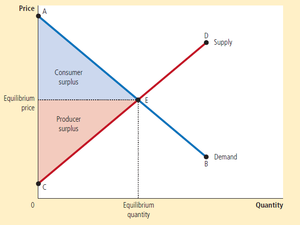
Graph
- On a supply and demand graph, the area of consumers surplus (CS) is below the demand curve but above the equilibrium price
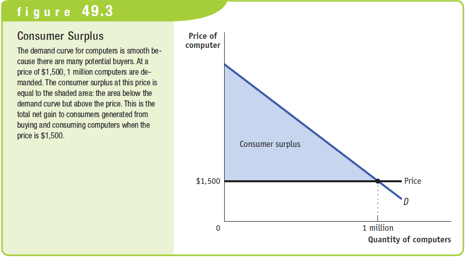
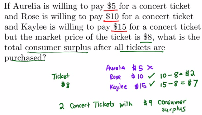
- Example 1
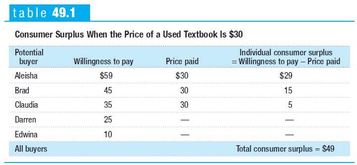
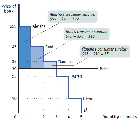
Example 2
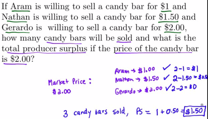
Producer Surplus
Meaning
- the difference between the price a sellers pays for and what he was actually willing to sell for
Graph
- On a supply and demand graph, the producer surplus is above the supply curve but below the equilibrium price.
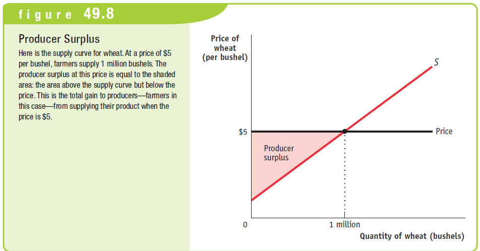
Example 1
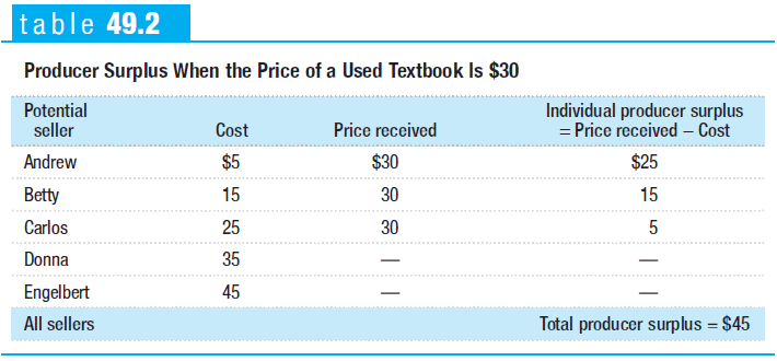
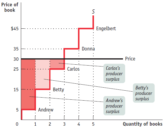
Example 2
Total Surplus
Meaning
- the sum of consumer and producer surplus
Graph
- the area between the supply and demand curves up to the equilibrium quantity
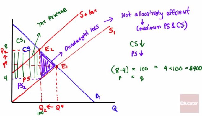
Effects of Taxes on Surplus
How does a tax affect hotel owners?
An excise tax on hotel owners will shift the supply curve to the left
The equilibrium price will be higher and the equilibrium quantity will be lower
How does a tax effect hotel guests
An excise tax on hotel guests will shift the demand curve to the left
The equilibrium price will be higher and the equilibrium quantity will be lower
The tax incidence in both cases are identical
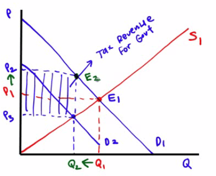
How the imposition of a tax will decrease consumer and producer surplus
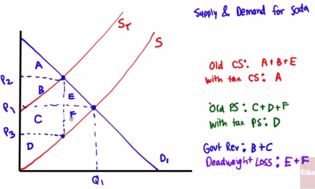
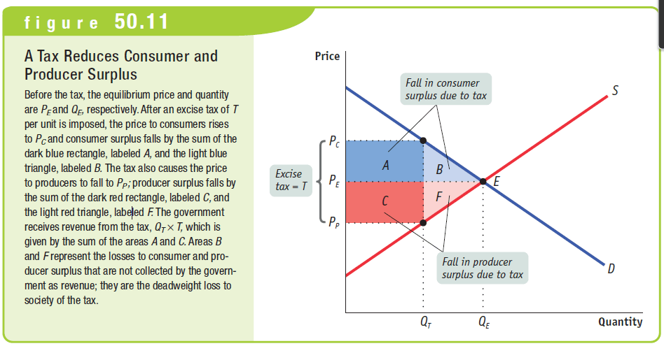
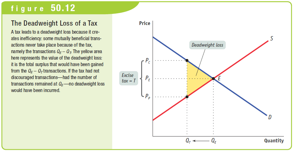
- Deadweight loss
International Trade
Autarky
- the quality of being self-sufficient with no imports or exports, a closed economy
Free trade and Tariffs
Free trade increases total surplus
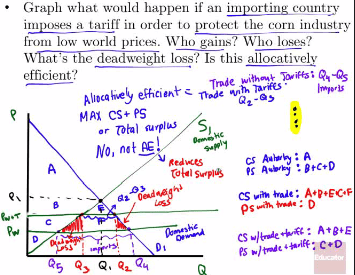
Tariffs serve to reduce allocative efficiency
Importing Countries
The World Price (Pw) will be below the autarky price and total surplus will increase
Domestic consumers gain, domestic producers lose, but the net gain is positive
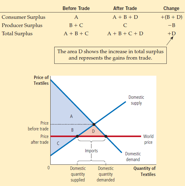
Buyers are better off (consumer surplus rises from A to A
- B + D)
Sellers are worse off (producer surplus falls from B + C to C)
Total surplus rises by an amount equal to area D
Trade raises the economic well-being of the country as a whole.
Exporting Countries
The World Price (Pw) will be above the autarky price and total surplus will increase
Domestic consumers lose, domestic producers gain, but the net gain is positive
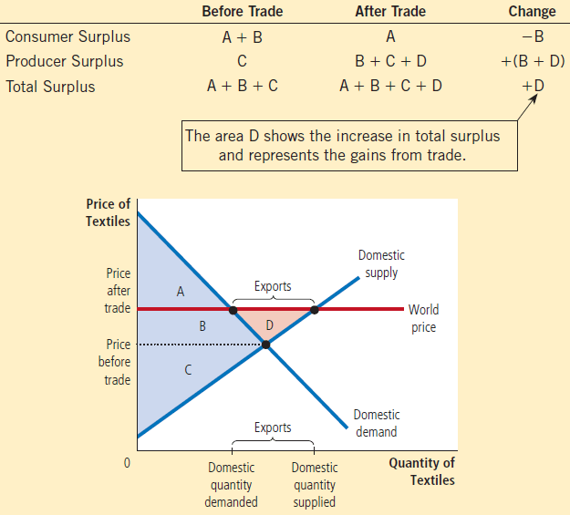
Sellers are better off (producer surplus rises from C to B
- C + D)
Buyers are worse off (consumer surplus falls from A + B to A)
Total surplus rises by an amount equal to area D
Trade raises the economic well-being of the country as a whole.
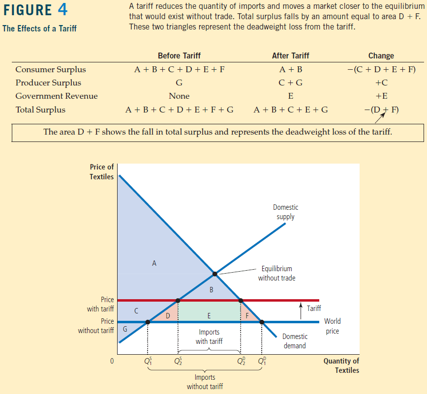
The Effects of a Tariff
Tariff
- a government tax on imports or exports
Example 1
Example 2